Mapping wildfire burn scars using HLS data
📥 Download GeospatialStudio-Walkthrough-BurnScars.ipynb and try it out
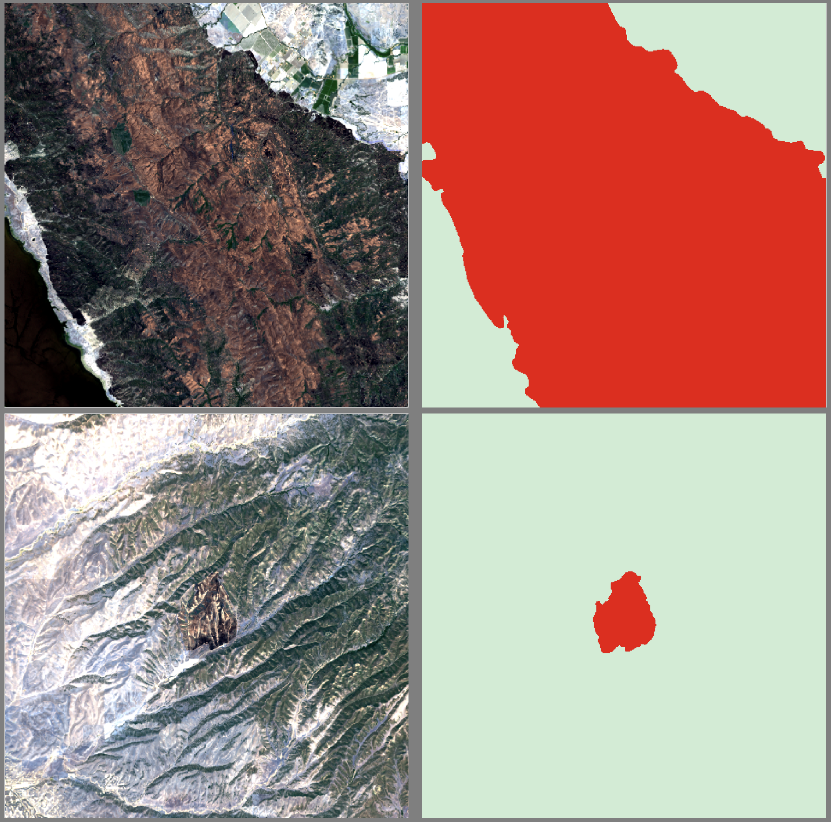
Imagine that you work in disaster response and need a rapid way to map the extent areas burned by wildfires. You need to do this in an automated, scalable manner. We can achieve this using an AI model which ingests satellite data (in this instance the NASA Harmonized Landsat Sentinel2 dataset) and outputs a map of burned area. We could potentially then integrate the burned area extent with details of infrastructure or assets to quantify impact.
In this walkthrough we will assume that a model doesn't exist yet and we want to train a new model. We will then show how to drive the model to map impact.
We will walk through the following steps as part of this walkthrough:
- Upload and onboarding of data
- Configuring and submitting a tuning task
- Monitoring model training
- Testing and validation of the outputs
Pre-requisites
This walkthrough assumes you have the data downloaded locally, it can be downloaded here: https://s3.us-east.cloud-object-storage.appdomain.cloud/geospatial-studio-example-data/burn-scar-training-data.zip
For more information about the Geospatial Studio see the docs page: Geospatial Studio Docs
For more information about the Geospatial Studio SDK and all the functions available through it, see the SDK docs page: Geospatial Studio SDK Docs
Get the training data
To train the AI model, we will need some training data which contains the input data and the labels (aka ground truth burn scar extent). To train our model we will use the following dataset: https://huggingface.co/datasets/ibm-nasa-geospatial/hls_burn_scars
We can download it here: https://s3.us-east.cloud-object-storage.appdomain.cloud/geospatial-studio-example-data/burn-scar-training-data.zip
Download and unzip the above archive and if you wish you can explore the data with QGIS (or any similar tool).
NB: If you already have the data in online you can skip this step.
# Import the required packages
import json
import rasterio
import matplotlib.pyplot as plt

import urllib3
urllib3.disable_warnings(urllib3.exceptions.InsecureRequestWarning)

from geostudio import Client
from geostudio import gswidgets
Connecting to the platform
First, we set up the connection to the platform backend. To do this we need the base url for the studio UI and an API key.
To get an API Key:
- Go to the Geospatial Studio UI page and navigate to the Manage your API keys link.
- This should pop-up a window where you can generate, access and delete your api keys. NB: every user is limited to a maximum of two activate api keys at any one time.
Store the API key and geostudio ui base url in a credentials file locally, for example in /User/bob/.geostudio_config_file. You can do this by:
echo "GEOSTUDIO_API_KEY=<paste_api_key_here>" > .geostudio_config_file
echo "BASE_STUDIO_UI_URL=<paste_ui_base_url_here>" >> .geostudio_config_file
Copy and paste the file path to this credentials file in call below.
#############################################################
# Initialize Geostudio client using a geostudio config file
#############################################################
gfm_client = Client(geostudio_config_file=".geostudio_config_file")
Data onboarding
In order to onboard your dataset to the Geospatial Studio, you need to have a direct download URL pointing to a zip file of the dataset. You can use Box, OneDrive or any other cloud storage you are used to, but in addition, to make this easier for you, there is a function which will upload your data to a temporary location in the cloud (with in Studio object storage) and provide you with a url which can be used to pass to the onboarding process. NB: the same upload function can be useful for pushing files for inferecnce or to processing pipelines.
If needed you can package a set of files for upload, you can use a command like:
zip -j burn-scars-upload.zip /Users/blair/Downloads/burn-scar-upload/*
# # (Optional) If you wish to upload the data archive through the studio, you can use this function. Copy the path to your zipped dataset below.
# uploaded_links = gfm_client.upload_file('../../../geobench-datasets/burn-scar-training-data.zip')
# uploaded_links
Onboard the dataset to the dataset factory
Now we use the SDK to provide the information about the dataset, including name, suffixes etc. A more detailed description of the dataset details is provided in the UI walkthrough. Here the SDK will do some basic sanity checks, and will (if possible) check that you have matching data and label pairs, and check that you have specified the correct number of bands. This creates dictionary with the required details, which you can then submit to the platform using the step below.
Note:
- Change the value of the
dataset_urlvariable below to the url of your zip file or thedownload_urllink you got from using the SDK upload_file function above - Change the values of
training_data_suffixandlabel_suffixto the suffixes of your training and label data files respectively if using a different dataset (aside from the one provided) - Change the
label_categories,custom_bandsand descriptions to those that match your dataset
# Explore datasets in the Studio

gfm_client.list_datasets(output="df")
# Copy the dataset_id of the dataset you want to explore further and replace with the dataset id below

gfm_client.get_dataset("geodata-yqesa6ozmzcuuauggkt9kq", output="json")
Onboard a new dataset
# Edit the details in the dict and dataset_url below to suit your dataset

dataset_url = 'https://s3.us-east.cloud-object-storage.appdomain.cloud/geospatial-studio-example-data/burn-scar-training-data.zip'

dataset_dict = {
    "purpose": "Segmentation",
    "dataset_url": dataset_url,
    "label_suffix": ".mask.tif",
    "dataset_name": "Burn Scars SDK demo",
    "description": "Burn Scars SDK data",
    "data_sources": [
        {
            "bands": [
                {"index": "0", "band_name": "Blue", "scaling_factor": 0.0001, "RGB_band": "B"},
                {"index": "1", "band_name": "Green", "scaling_factor": 0.0001, "RGB_band": "G"},
                {"index": "2", "band_name": "Red", "scaling_factor": 0.0001, "RGB_band": "R"},
                {"index": "3", "band_name": "NIR_Narrow", "scaling_factor": 0.0001},
                {"index": "4", "band_name": "SWIR1", "scaling_factor": 0.0001},
                {"index": "5", "band_name": "SWIR2", "scaling_factor": 0.0001}
            ],
            "connector": "sentinelhub",
            "collection": "hls_l30",
            "file_suffix": "_merged.tif",
            "modality_tag": "HLS_L30"
        }
    ],
    "label_categories": [
        {"id": "-1", "name": "Igone", "color": "#000000", "opacity": "0", "weight": None},
        {"id": "0", "name": "NoData", "color": "#000000", "opacity": "0", "weight": None},
        {"id": "1", "name": "BurnScar", "color": "#ea7171", "opacity": 1, "weight": None}
    ],
    "version": "v2"
}
# start onboarding process

onboard_response = gfm_client.onboard_dataset(dataset_dict)
display(json.dumps(onboard_response, indent=2))
# Poll onboarding status
gfm_client.poll_onboard_dataset_until_finished(onboard_response["dataset_id"])
Fine-tuning submission
Once the data is onboarded, you are ready to setup your tuning task. In order to run a fine-tuning task, you need to select the following items:
- tuning task type - what type of learning task are you attempting? segmentation, regression etc
- fine-tuning dataset - what dataset will you use to train the model for your particular application?
- base foundation model - which geospatial foundation model will you use as the starting point for your tuning task?
Below we walk you through how to use the Geospatial Studio SDK to see what options are available in the platform for each of these, then once you have made your selection, how we configure our task and submit it.
Tuning task
The tuning task tells the model what type of task it is (segmentation, regression etc), and exposes a range of optional hyperparameters which the user can set. These all have reasonable defaults, but it gives uses the possibility to configure the model training how they wish. Below, we will check what task templates are available to us, and then update some parameters.
Advanced users can create and upload new task templates to the platform, and instructions are found in the relevant notebook and documentation. The templates are for Terratorch (the backend tuning library), and more details of Terratroch and configuration options can be found here: https://ibm.github.io/terratorch/
tasks = gfm_client.list_tune_templates(output="df")
display(tasks[['name','description', 'id','created_by','updated_at']])
# Choose a task from the options above.  Copy and paste the id into the variable, tid, below.
task_id = 'e4791b2c-bb17-4a5e-9f05-1be5411a4fa6'
# Now we can view the full meta-data and details of the selected task
task_meta = gfm_client.get_task(task_id, output="df")
task_meta
If you are happy with your choice, you can decide which (if any) hyperparameters you want to set (otherwise defaults will be used).
Here we can see the available parameters and their associated defaults. To update a parameter you can just set values in the dictionary (as shown below for max_epochs).
task_params = gfm_client.get_task_param_defaults(task_id)
task_params
task_params['runner']['max_epochs'] = '2'
task_params['optimizer']['type'] = 'AdamW'
task_params['data']['batch_size'] = 4
Base foundation model
The base model is the foundation model (encoder) which has been pre-trained and has the basic understanding of the data. More information can currently be found on the different models in the documentation.
base = gfm_client.list_base_models(output='df')
display(base[['name','description','id','updated_at']])
# copy and paste the id of the base model you wish to use

base_model_id = 'f24fad3d-d5b5-40aa-a8ce-700a1a3d0a83'
Submitting the tune
Now we pull these choices together into a payload which we then submit to the platform. This will then deploy the job in the backend and we will see below how we can monitor it. First, we populate the payload so we can check it, then we simply submit.
# create the tune payload

dataset_id = onboard_response["dataset_id"] # the dataset_id of the dataset you onboarded above

tune_payload = {
  "name": "burn-scars-demo",
  "description": "Segmentation",
  "dataset_id": dataset_id,
  "base_model_id": base_model_id,
  "tune_template_id": task_id,
  "model_parameters": task_params # uncomment this line if you customised task_params in the cells above otherwise, defaults will be used
}

print(json.dumps(tune_payload, indent=2))
submitted = gfm_client.submit_tune(
        data = tune_payload,
        output = 'json'
)

print(submitted)
Monitoring training
Once the tune has been submitted you can check its status and monitor tuning progress through the SDK. You can also access the training metrics and images in MLflow. The get_tune function will give you the meta-data of the tune, including the status.
# Poll fine tuning status
gfm_client.poll_finetuning_until_finished(tune_id=submitted["tune_id"])
tune_id = submitted["tune_id"]

tune_info = gfm_client.get_tune(tune_id, output='df')
tune_info
Once it has started training, you will also be able to access the training metrics. The get_tune_metrics_df function returns a dataframe containing the up-to-date training metrics, which you are free to explore and analyse. In addition to that, you can simply plot the training and validation loss and multi-class accuracy using the plot_tune_metrics function.
gfm_client.get_tune_metrics_df(tune_id)
gswidgets.plot_tune_metrics(client=gfm_client, tune_id=tune_id)
Once your model is finished training and you are happy with the metrics (and images in MLflow), you can run some inference in test mode through the inference service.
Testing your model
To do a test deployment and inference with the model, we need to register the model with the inference service. To do this you need to select a model style (describing the visulisation style of the model output), and define the data required to feed the model (in the example here it is using Sentinel Hub). For the data specification, you need to define the data collection and bands from sentinelhub (using the collection and band names for SH). In addition, if the data to be fed in is returned from SH with a scale factor that needs to be added here too. Data collection data for HLS are found here: https://docs.sentinel-hub.com/api/latest/data/hls/
Example test locations
| Location | Date | Bounding box |
|---|---|---|
| Park Fire, CA, USA (Cohasset, CA) | 2024-08-12 | [-121.837006, 39.826468, -121.641312, 40.038655] |
| Rhodes, Greece | 2023-08-01 | [27.91, 35.99, 28.10, 36.25] |
| Rafina, Greece | 2018-08-04 | [23.92, 38.00, 24.03, 38.08] |
| Bandipura State Forest, Karnataka, India | 2019-02-26 | [76.503245, 11.631803, 76.690118, 11.762633] |
| Amur Oblast fires, Russia | 2018-05-29 | [127.589722, 54.055357, 128.960266, 54.701614] |
Try out the model for inference
Once your model has finished tuning, if you want to run inference as a test you can do by passing either a location (bbox) or a url to a pre-prepared files. The steps to test the model are:
- Define the inference payload
- Try out the tune temporarily
# define the inference payload

bbox = [-121.837006,39.826468,-121.641312,40.038655]

request_payload = {
	"description": "Park Fire 2024 SDK",
	"location": "Red Bluff, California, United States",
	"spatial_domain": {
			"bbox": [bbox],
			"polygons": [],
			"tiles": [],
			"urls": []
	},
	"temporal_domain": [
			"2024-08-12_2024-08-13"
	]
}
Once you have defined your inference payload, you can now run it with a test inference. As with the main inference service, this is done by either supplying a bounding box (bbox), time range (start_date, end_date) and the model_id. You can then monitor it and visualise the outputs either through the SDK, or in the UI.
# Now submit the test inference request
inference_response = gfm_client.try_out_tune(tune_id=tune_id, data=request_payload)
inference_response
Monitoring your inference task
Once submitted you can check on progress using the following function which will return all the metadata about the inference task, including the status. You can optionally use the poll_until_finished to watch the status until it completes. For a test inference it can take 5-10 minutes, depending on the size of the data query, the size of the model etc.
gfm_client.get_inference(inference_response['id'], output="df")
# Poll inference status
gfm_client.poll_inference_until_finished(inference_id=inference_response['id'], poll_frequency=10)
Accessing inference outputs
Once an inference run is completed, the inputs and outputs of each task within an inference are packaged up into a zip file which is uploaded to a url you can use to download the files.
To access the inference task files:
- Get the inference tasks list
- Identify the specific inference task you want to view
- Download task output files
# Get the inference tasks list
inf_tasks_res = gfm_client.get_inference_tasks(inference_response["id"])
inf_tasks_res
df = gfm_client.inference_task_status_df(inference_response["id"])


display(df.style.map(gswidgets.color_inference_tasks_by_status))
gswidgets.view_inference_process_timeline(gfm_client, inference_id = inference_response["id"])
Next, Identify the task you want to view from the response above, ensure status of the task is FINISHED and set selected_task variable below to the task number at the end of the task id string. For example, if task_id is "6d1149fa-302d-4612-82dd-5879fc06081d-task_0", selected_task woul be 0
# Select a task to view

selected_task = 0
selected_task_id = f"{inference_response["id"]}-task_{selected_task}"
# Download task output files

gswidgets.fileDownloaderTasks(client=gfm_client, task_id=selected_task_id)
Visualizing the output of the inference runs
You can check out the results visually in the Studio UI, or with the quick widget below. You can alternatively use the SDK to download selected files for further analysis see documentation.
We have several options for visualising the data:
- we can load the data with a package like rasterio and plot the images, and/or access the values.
- we could use the widget from the SDK to visualise the chosen files for a inference run. (shown below)
- view the data in the Geospatial Studio Inference lab UI.
- load the files in an external software, such as QGIS.
Load the data with a package rasterio and plot the images, and/or access the values.
# Paste the name (+path) to one of the files you downloaded and select the band you want to load+plot
filename = '9a0588de-8858-4c31-8c6d-91b9c74333d1-task_0_HLS_L30_2024-08-12__merged.tif.tif'
band_number = 1

# open the file and read the band and metadata with rasterio
with rasterio.open(filename) as fp:
    data = fp.read(band_number)
    bounds = fp.bounds


print("Image dimensions: " + str(data.shape))

plt.imshow(data, extent=[bounds.left, bounds.right, bounds.bottom, bounds.top])
plt.xlabel('Longitude'); plt.xlabel('Latitude')
Visualize through the SDK widgets
# Visualize output files with the SDK
gswidgets.inferenceTaskViewer(client=gfm_client, task_id=selected_task_id)