Mapping flooding using an AI flood model
📥 Download GeospatialStudio-Walkthrough-Flooding.ipynb and try it out
Assume you are interested in mapping flooding, traditionally you might have either relied on on-the-ground mapping, or possibly for manual analysis of remote-sensing imagery (i.e. satellite or UAV). In order to scale up these efforts and operationalise, we need a way to automate the extraction of flood extent from satellite imagery. This is where we turn to AI models.
The model you will use in this walkthrough was fine-tuned from the Prithvi foundation model and using the Sen1Floods11 dataset link here.
In this walkthrough we will assume that a model doesn't exist yet and we want to train a new model. We will then show how to drive the model to map impact.
We will walk through the following steps as part of this walkthrough:
- Upload and onboarding of data
- Configuring and submitting a tuning task
- Monitoring model training
- Testing and validation of the outputs
Pre-requisites
You will require access to an instance of the Geospatial Studio. For more information about the Geospatial Studio see the docs page: Geospatial Studio Docs
For more information about the Geospatial Studio SDK and all the functions available through it, see the SDK docs page: Geospatial Studio SDK Docs
This walkthrough also requires you to have a direct download URL pointing to a zip file of the dataset you wish to use. We provide a sample dataset url (zip file) below to go through this notebook. If you have the dataset locally, you can find instructions on how to use the SDK to temporarily upload it to the cloud and create a download url link in the steps that follow.
Get the training data
To train the AI model, we will need some training data which contains the input data and the labels (aka ground truth flooding extent). To train our model we will use the following dataset: https://geospatial-studio-example-data.s3.us-east.cloud-object-storage.appdomain.cloud/sen2_flood_dst.zip
Download and unzip the above archive and if you wish you can explore the data with QGIS (or any similar tool).
NB: If you already have the data in online you can skip this step.
%load_ext autoreload
%autoreload 2
import os
import json
import uuid
import pandas as pd
import rasterio
from rasterio.plot import show
import matplotlib.pyplot as plt

import urllib3
urllib3.disable_warnings(urllib3.exceptions.InsecureRequestWarning)

from geostudio import Client
from geostudio import gswidgets
Connecting to the platform
First, we set up the connection to the platform backend. To do this we need the base url for the studio UI and an API key.
To get an API Key:
- Go to the Geospatial Studio UI page and navigate to the Manage your API keys link.
- This should pop-up a window where you can generate, access and delete your api keys. NB: every user is limited to a maximum of two activate api keys at any one time.
Store the API key and geostudio ui base url in a credentials file locally, for example in /User/bob/.geostudio_config_file. You can do this by:
echo "GEOSTUDIO_API_KEY=<paste_api_key_here>" > .geostudio_config_file
echo "BASE_STUDIO_UI_URL=<paste_ui_base_url_here>" >> .geostudio_config_file
Copy and paste the file path to this credentials file in call below.
#############################################################
# Initialize Geostudio client using a geostudio config file
#############################################################
gfm_client = Client(geostudio_config_file=".geostudio_config_file")
Data onboarding
In order to onboard your dataset to the Geospatial Studio, you need to have a direct download URL pointing to a zip file of the dataset. You can use this dataset url as an example to go through this notebook.
If you have the dataset locally, you can use Box, OneDrive or any other cloud storage you are used to, but in addition, to make this easier for you, there is a function which will upload your data to a temporary location in the cloud (with in Studio object storage) and provide you with a url which can be used to pass to the onboarding process. NB: the same upload function can be useful for pushing files for inferecnce or to processing pipelines.
If needed you can package a set of files for upload, you can use a command like:
zip -j flooding-dataset-upload.zip /Users/beldinemoturi/Downloads/flooding-dataset-upload/*
# (Optional) If you wish to upload the data archive through the studio, you can uncomment and use this function.
uploaded_links = gfm_client.upload_file('/Users/beldinemoturi/Downloads/flooding_dataset.zip')
uploaded_links
Onboard the dataset to the dataset factory
Now we use the SDK to provide the information about the dataset, including name, suffixes etc. A more detailed description of the dataset details is provided in the UI walkthrough. Here the SDK will do some basic sanity checks, and will (if possible) check that you have matching data and label pairs, and check that you have specified the correct number of bands. This creates dictionary with the required details, which you can then submit to the platform using the step below.
Note:
- Change the value of the
dataset_urlvariable below to the url of your zip file or thedownload_urllink you got from using the SDK upload_file function above - Change the values of
training_data_suffixandlabel_suffixto the suffixes of your training and label data files respectively if using a different dataset (aside from the one provided) - Change the
label_categories,custom_bandsand descriptions to those that match your dataset
uploaded_links["download_url"]
# Edit the dict below to suit your dataset details.

dataset_dict = {
    "dataset_name": "Sentinel Flood Multimodal",
    "data_sources": [
        {
            "bands": [
                {"index":"0", "band_name": "Coastal_aerosol", "RGB_band": "R", "description": ""},
                {"index":"1", "band_name": "Blue", "RGB_band": "G", "description": ""},
                {"index":"2", "band_name": "Green", "RGB_band": "B", "description": ""},
                {"index":"3", "band_name": "Red", "description": ""},
                {"index":"4", "band_name": "05_-_Vegetation_Red_Edge", "description": ""},
                {"index":"5", "band_name": "06_-_Vegetation_Red_Edge", "description": ""},
                {"index":"6", "band_name": "07_-_Vegetation_Red_Edge", "description": ""},
                {"index":"7", "band_name": "08_-_NIR", "description": ""},
                {"index":"8", "band_name": "08A_-_Vegetation_Red_Edge", "description": ""},
                {"index":"9", "band_name": "09_-_Water_vapour", "description": ""},
                {"index":"10", "band_name": "11_-_SWIR", "description": ""},
                {"index":"11", "band_name": "12_-_SWIR", "description": ""},
                {"index":"12", "band_name": "Cloud_Probability", "description": ""}
            ],
            "connector": "sentinelhub",
            "collection": "s2_l2a",
            "modality_tag": "S2L1C",
            "file_suffix": "_S2Hand.tif",
            "scaling_factor": [1, 1, 1, 1, 1, 1]
        },
        {
            "bands": [
                {"index":"0", "band_name": "VV (Gray)", "description": ""},
                {"index":"1", "band_name": "VH", "description": ""}
            ],
            "connector": "sentinelhub",
            "collection": "s1_grd",
            "modality_tag": "S1GRD",
            "align_dates": "true",
            "file_suffix": "_S1Hand.tif",
            "scaling_factor": [1, 1]
        }
    ],
    "label_categories": [
        {"id": "0", "name": "No Floods", "description": "Flooding assets"},
        {"id": "1", "name": "Floods", "description": "Flooding assets"}
    ],
    "dataset_url": uploaded_links["download_url"],
    "description": "Flood data from places",
    "label_suffix": "_LabelHand.tif",
    "purpose": "Segmentation"
}
Pre-scan the dataset
Pre-scan the dataset to check the accessibility of the dataset URL, ensure corresponding data and label files are present, and extract bands and their descriptions from the dataset.
# [Optional]

gfm_client.pre_scan_dataset({
  "dataset_url": uploaded_links["download_url"],
  "label_suffix": "_LabelHand.tif",
  "training_data_suffixes":
    ["_S2Hand.tif", "_S1Hand.tif"]
})
# start onboarding process

onboard_response = gfm_client.onboard_dataset(data=dataset_dict)
display(json.dumps(onboard_response, indent=2))
Fine-tuning submission
Once the data is onboarded, you are ready to setup your tuning task. In order to run a fine-tuning task, you need to select the following items:
- tuning task type/config template - what type of learning task are you attempting? segmentation, regression etc
- fine-tuning dataset - what dataset will you use to train the model for your particular application?
- base foundation model - which geospatial foundation model will you use as the starting point for your tuning task?
Below we walk you through how to use the Geospatial Studio SDK to see what options are available in the platform for each of these, then once you have made your selection, how we configure our task and submit it.
Tuning task
The tuning task tells the model what type of task it is (segmentation, regression etc), and exposes a range of optional hyperparameters which the user can set. These all have reasonable defaults, but it gives uses the possibility to configure the model training how they wish. Below, we will check what task templates are available to us, and then update some parameters.
Advanced users can create and upload new task templates to the platform, and instructions are found in the relevant notebook and documentation. The templates are for Terratorch (the backend tuning library), and more details of Terratroch and configuration options can be found here: https://ibm.github.io/terratorch/
# list tasks available

tasks = gfm_client.list_tune_templates(output="df")
display(tasks[['name','description', 'id','created_by','updated_at']])
# Choose a task from the options above.  Copy and paste the id into the variable, task_id, below. For this example, it is a segmentation task since we are classifying flooded and non-flooded areas
task_id = '48c878d8-3b05-4ca5-bd89-89400c8790eb'
# view the full meta-data and details of the selected task
task_meta = gfm_client.get_task(task_id)
task_meta
If you are happy with your choice, you can decide which (if any) hyperparameters you want to set (otherwise defaults will be used).
Here we can see the available parameters and their associated defaults. To update a parameter you can just set values in the dictionary (as shown below for max_epochs).
# show the default values for parameters

task_params = gfm_client.get_task_param_defaults(task_id)
task_params
# configure the parameters you want

task_params['runner']['max_epochs'] = '3'
# task_params['optimizer']['type'] = 'AdamW'
# task_params['data']['batch_size'] = 4
Base foundation model
The base model is the foundation model (encoder) which has been pre-trained and has the basic understanding of the data. More information can currently be found on the different models we have open-sourced on hugging face.
# list foundation models available

base = gfm_client.list_base_models(output='df')
display(base[['name','description','id','updated_at']])
# select base foundation model
base_model_id = '55e638d9-7a7c-4e8b-bda2-035b172922af'
Submitting the tune
Now we pull these choices together into a payload which we then submit to the platform. This will then deploy the job in the backend and we will see below how we can monitor it. First, we populate the payload so we can check it, then we simply submit.
# create the tune payload

dataset_id = "geodata-zvgkj5qqwxbhzzz25qbuxz" # the dataset_id of the dataset you onboarded above

tune_payload = {
  "name": "test-fine-tuning-multimodal",
  "description": "Segmentation",
  "dataset_id": dataset_id,
  "base_model_id": base_model_id,
  "tune_template_id": task_id,
}

print(json.dumps(tune_payload, indent=2))
# submit tune

submitted = gfm_client.submit_tune(
        data = tune_payload,
        output = 'json'
)

print(submitted)
Monitoring training
Once the tune has been submitted you can check its status and monitor tuning progress through the SDK. You can also access the training metrics and images in MLflow. The get_tune function will give you the meta-data of the tune, including the status.
# get metadata about the submitted tune

tune_id = submitted.get("tune_id")

tune_info = gfm_client.get_tune(tune_id, output='json')
tune_info
Once the model has started training, you will also be able to access the training metrics. The get_tune_metrics_df function returns a dataframe containing the up-to-date training metrics, which you are free to explore and analyse. In addition to that, you can simply plot the training and validation loss and multi-class accuracy using the plot_tune_metrics function.
# get training metrics

mdf = gfm_client.get_mlflow_metrics("geotune-iskjtu463hxou9mukjct9o")
mdf.head()
# plot some basic training metrics

# gfm_client.plot_tune_metrics(tune_id)
Once your model is finished training and you are happy with the metrics (and images in MLflow), you can run some inference in test mode through the inference service.
Testing your model
To do a test deployment and inference with the model, we need to register the model with the inference service. To do this you need to select a model style(describing the visulisation style of the model output), and define the data required to feed the model (in the example here it is using Sentinel Hub). For the data specification, you need to define the data collection and bands from sentinelhub (using the collection and band names for SH). In addition, if the data to be fed in is returned from SH with a scale factor that needs to be added here too. Data collection data for HLS are found here: https://docs.sentinel-hub.com/api/latest/data/hls/
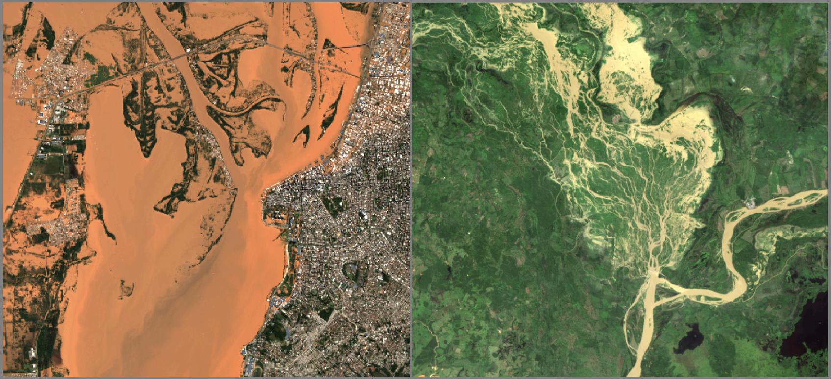
Example flood events
| Location | Date | Bounding box | Link |
|---|---|---|---|
| Maiduguri, Nigeria | 2024-09-12 | [13.146418, 11.799808, 13.215874, 11.871586] | https://www.aljazeera.com/features/2024/9/19/a-disaster-homes-lost-relatives-missing-in-floods-in-northeast-nigeria |
| Porto Alegre, Brazil | 2024-05-06 | [-51.33225, -30.08903, -51.19011, -29.97489] | https://www.reuters.com/pictures/stunning-images-show-extent-flooding-southern-brazil-2024-05-07/ |
| Ahero, Kenya | 2024-05-05 | [34.838652, -0.231379, 34.977847, -0.131439] | |
| Gloucester, UK | 2024-01-09 | [-2.311807, 51.855573, -2.17892, 51.952735] |
Try out the model for inference
Once your model has finished tuning, if you want to run inference as a test you can do by passing either a location (bbox) or a url to a pre-prepared files. The steps to test the model are:
- Define the inference payload
- Try out the tune temporarily
# define the inference payload

bbox = [92.40665153547121, 26.1051042015407,92.92535070071905,26.498933088370826]

request_payload = {
	"description": "Jarani, Nagaon, Nagaon, Assam, India",
	"location": "Jarani, Nagaon, Nagaon, Assam, India",
	"spatial_domain": {
			"bbox": [bbox],
			"polygons": [],
			"tiles": [],
			"urls": []
	},
	"temporal_domain": [
			"2024-07-25_2024-07-27"
	]
}
Once you have registered the model, you can now run it with a test inference. As with the main inference service, this is done by either supplying a bounding box (bbox), time range (start_date, end_date) and the model_id. You can then monitor it and visualise the outputs either through the SDK, or in the UI.
# Now submit the test inference request
inference_response = gfm_client.try_out_tune(tune_id=tune_id, data=request_payload)
inference_response
Monitoring your inference task
Once submitted you can check on progress using the following function which will return all the metadata about the inference task, including the status. You can optionally use the poll_until_finished to watch the status until it completes. For a test inference it can take 5-10 minutes, depending on the size of the data query, the size of the model etc.
# get metadata about the inference task

gfm_client.get_inference(inference_response['id'])
Checking model outputs
You can check out the results visually in the Studio UI, or with the quick widget below. You can alternatively use the SDK to download selected files for further analysis see documentation.
Note:
For now, you can check out the inference output and results visually in the Studio UI through the history tab of the inference page.
# view inference results

# gswidgets.inferenceViewer(gfm_client, inference_response['id'])