Lab 6¶

🌍 Geospatial Exploration and Orchestration Studio¶

Training a Custom Model for Floods Detection¶

License
TerraStackAI
Built With
Deployment

---

1.0 Introduction¶

Welcome to this hands-on workshop on floods detection using the Geospatial Studio! This tutorial will guide you through the complete workflow of fine-tuning a geospatial foundation model and running inference to detect floods from satellite imagery.

What you'll learn:

• Setting up and connecting to the Geospatial Studio platform
• Fine-tuning models for floods segmentation tasks with pre-trained foundation models and datasets
• Running inference on real-world wildfire data (Park Fire, California)
• Visualizing and analyzing results in the Studio UI
• Comparing results with a better trained model

Prerequisites:

• A deployed instance of the Geospatial Studio
• Access to GPU resources (for fine-tuning section)
• Basic familiarity with Python and Jupyter notebooks

1.0.1 Understanding the Workflow¶

Before we begin, the complete workflow will be as follows:

Key Components:

1. Foundation Model (Backbone): Pre-trained model with general geospatial understanding
2. Training Dataset: Labeled data for your specific task
3. Task Template: Configuration defining the learning task
4. Fine-tuning Job: Training process that customizes the model
5. Trained Model (Tune): Your custom model checkpoint
6. Inference: Running predictions on new data

---

1.0.2 Example: floods Detection Workflow¶

Below is an example of what you'll achieve in this workshop - detecting floodss from satellite imagery using fine-tuned geospatial foundation models.

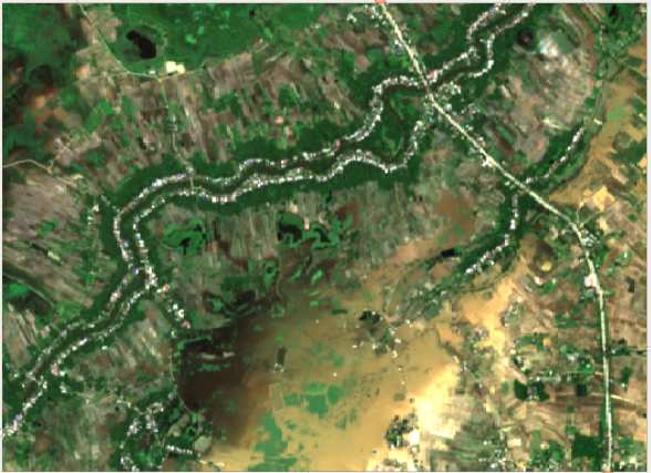
Input Satellite Imagery¶

Raw satellite data showing the area affected by wildfire:

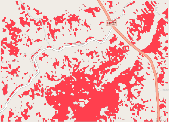
Model Prediction¶

The fine-tuned model identifies floods areas:

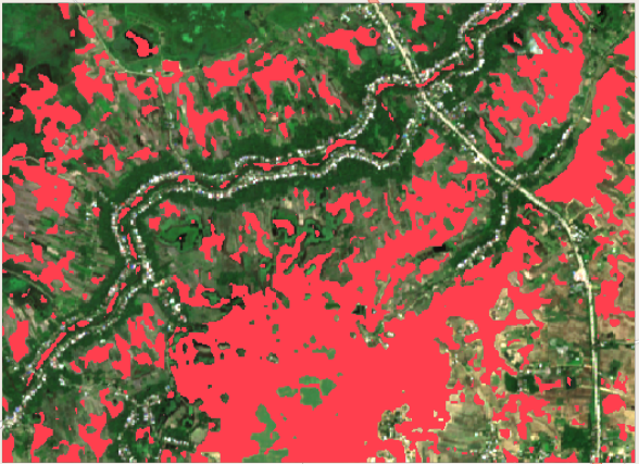
Prediction Overlay¶

floods predictions overlaid on the original imagery for validation:

This workflow demonstrates the power of geospatial foundation models in identifying and mapping wildfire-affected areas, which is crucial for disaster response, environmental monitoring, and recovery planning.

Let's get started by setting up your environment and connecting to the platform!

1.1 Set up and Installation¶

1.1.0 Prerequisites¶

Create a python environment

python -m venv venv 
OR # depending on your available python version
python3 -m venv venv
source venv/bin/activate

Install geostudio sdk

pip install geostudio

Set the jupyter notebook kernel to point to the above created python environment.

1.1.1 Import required packages¶

In [ ]:

%load_ext autoreload
%autoreload 2

%load_ext autoreload %autoreload 2

In [ ]:

# Import the required packages
import json
import urllib3
urllib3.disable_warnings(urllib3.exceptions.InsecureRequestWarning)
from geostudio import Client

# Import the required packages import json import urllib3 urllib3.disable_warnings(urllib3.exceptions.InsecureRequestWarning) from geostudio import Client

1.2 Connecting to the platform¶

First, we set up the connection to the platform backend. To do this we need the base url for the studio UI and an API key.

To get an API Key:

1. Go to the provided cluster url of the deployed version of the Geospatial Studio UI page [hrl to be provided here] and navigate to the Manage your API keys link.
2. This should pop-up a window where you can generate, access and delete your api keys. NB: every user is limited to a maximum of two activate api keys at any one time.

Store the API key and geostudio ui base url in a credentials file locally, for example in /User/bob/.geostudio_config_file. You can do this by:

echo "GEOSTUDIO_API_KEY=<paste_api_key_here>" > .geostudio_config_file
echo "BASE_STUDIO_UI_URL=<paste_ui_base_url_here>" >> .geostudio_config_file

Copy and paste the file path to this credentials file in call below. You will need to ensure that the geostudio_config_file is accessible and correctly configured. If you encounter any issues, please verify the file path and contents of the .geostudio_config_file to ensure they are accurate and up-to-date.

In [ ]:

#############################################################
# Initialize Geostudio client using a geostudio config file
#############################################################
gfm_client = Client(geostudio_config_file=".geostudio_config_file")

############################################################# # Initialize Geostudio client using a geostudio config file ############################################################# gfm_client = Client(geostudio_config_file=".geostudio_config_file")

2.0 Multimodal Floods dataset¶

2.1 Reviewing already prepared and onboarded Multimodal floods dataset¶

In this section, we'll explore how to review datasets that have already been prepared and onboarded to the Geospatial Studio. This is useful for understanding what data is available before starting a fine-tuning task.

In [ ]:

from pandas import DataFrame

# List all available datasets in the studio
datasets = gfm_client.list_datasets()['results']
display(DataFrame(datasets))

from pandas import DataFrame # List all available datasets in the studio datasets = gfm_client.list_datasets()['results'] display(DataFrame(datasets))

In [ ]:

# Get detailed information about a specific floodss dataset
# If you know the dataset name or ID, you can retrieve its details
floods_dataset_id = "geodata-4vdk3x6pyfvr59zxki6kcc"
floods_dataset_id

# Get detailed information about a specific floodss dataset # If you know the dataset name or ID, you can retrieve its details floods_dataset_id = "geodata-4vdk3x6pyfvr59zxki6kcc" floods_dataset_id

In [ ]:

# Get detailed metadata for a specific dataset
# Replace with your actual dataset_id from the list above
dataset_details = gfm_client.get_dataset(floods_dataset_id)
print(json.dumps(dataset_details, indent=2))

# Get detailed metadata for a specific dataset # Replace with your actual dataset_id from the list above dataset_details = gfm_client.get_dataset(floods_dataset_id) print(json.dumps(dataset_details, indent=2))

From the above output, the dataset Configuration is:

• Data Sources: 2 modalities (S2L2A and S1GRD)
  • Sentinel-2 L2A (S2L2A): 13 spectral bands (B01-B12, CLD)
  • Sentinel-1 GRD (S1GRD): 2 SAR bands (VV, VH)
• 2 label categories: No Floods (0) Floods (1)
• File format: GeoTIFF with ._LabelHand.tif suffix for labels
• Purpose: Segmentation (pixel-level classification)
• Size: 1.8GB

3.0 Run a model training job¶

To ran a Finetuning job, we need:

• A base model
• A dataset
• A task template

---

3.1 Select a Base Model¶

---

For this task, we will use the TerraMind-1.0-tiny foundation model as our base model.

About TerraMind-1.0-tiny:

• Large-scale generative multimodal model for Earth observation
• Symmetric Transformer-based encoder-decoder architecture
• Trained on multiple modalities:
  • Optical imagery (Sentinel-2)
  • Radar data (Sentinel-1 SAR)
  • Digital Elevation Model (DEM)
  • Land Use/Land Cover (LULC)
  • Vegetation indices (NDVI)
  • Geographic metadata and text captions
• Uses dual-scale pretraining on both pixel-level and token-level representations
• Trained on 9 million samples from Copernicus Sentinel missions
• Supports any-to-any generation and multi-scale features
• Optimized for zero-shot and fine-tuning on downstream tasks

The backbone configuration includes:

• Model architecture: Symmetric Transformer encoder-decoder
• Tokenization: Discrete tokens for multimodal inputs
• Pre-training: Dual-scale (pixel + token level)
• Model family: TerraMind by IBM Research & ESA

In [ ]:

# List all the base models onboarded in the cluster
base_models = gfm_client.list_base_models()['results']
display(DataFrame(base_models))

# Select Terramind Tiny model
terramind_tiny_base_model_id = "fdf47e1e-aa27-42c2-b5da-b82e8f608c9d"

# List all the base models onboarded in the cluster base_models = gfm_client.list_base_models()['results'] display(DataFrame(base_models)) # Select Terramind Tiny model terramind_tiny_base_model_id = "fdf47e1e-aa27-42c2-b5da-b82e8f608c9d"

---

3.2 Select a task template¶

---

A task template defines:

• The type of ML task (segmentation, regression, classification)
• Model architecture options
• Training hyperparameters
• Default configurations

Why Do We Need It?¶

When you upload a model checkpoint, GEOStudio needs to know:

1. What task the model was trained for
2. How to configure the model for inference
3. What inputs the model expects

Available Task Types¶

• Segmentation - Pixel-wise classification (floods, floodss, land cover)
• Regression - Continuous value prediction (biomass, temperature)
• Classification - Image-level labels (crop type, building detection)
• User-Defined - Specific User defined templates for specific model use cases (convnext-template)

For this example, we will be using the ** terramind Segmentation** task type.

In [ ]:

# List all the templates onboarded in the cluster
tune_templates = gfm_client.list_tune_templates()['results']
display(DataFrame(tune_templates))

# Select segmentation template
terramind_segmentation_template_id = "ccf91f72-0a17-41f0-b835-5be3c901fe34"

# List all the templates onboarded in the cluster tune_templates = gfm_client.list_tune_templates()['results'] display(DataFrame(tune_templates)) # Select segmentation template terramind_segmentation_template_id = "ccf91f72-0a17-41f0-b835-5be3c901fe34"

---

3.3 Submit the training job¶

---

• Base Model: TerraMind-1.0-tiny (300M parameters)
• Dataset: floods training data
• Task Template: Segmentation template
• Name: floods-demo

In [ ]:

# Create the fine-tuning payload
payload = {
    "name": "terramind_tiny-demo",
    "description": "Segmentation model for multimodal floods detection",
    "dataset_id": floods_dataset_id,
    "base_model_id": terramind_tiny_base_model_id,
    "tune_template_id": terramind_segmentation_template_id,
    "model_parameters": {
        "runner": {
        "max_epochs": 2
            }
   }
}

print("📋 Fine-Tuning Configuration:")
print(json.dumps(payload, indent=2))

# Create the fine-tuning payload payload = { "name": "terramind_tiny-demo", "description": "Segmentation model for multimodal floods detection", "dataset_id": floods_dataset_id, "base_model_id": terramind_tiny_base_model_id, "tune_template_id": terramind_segmentation_template_id, "model_parameters": { "runner": { "max_epochs": 2 } } } print("📋 Fine-Tuning Configuration:") print(json.dumps(payload, indent=2))

In [ ]:

# Submit the fine-tuning job
print("\n🚀 Submitting fine-tuning job...\n")

tune_submitted = gfm_client.submit_tune(payload, output='json')

print("✅ Fine-tuning job submitted successfully!")
print(json.dumps(tune_submitted, indent=2))

# Save the tune ID for later use
tune_id = tune_submitted['tune_id']
print(f"\n📌 Tune ID: {tune_id}")
print("\nYou can monitor progress in the Studio UI under 'Start fine-tuning' > 'Model & Tunes'")

# Submit the fine-tuning job print("\n🚀 Submitting fine-tuning job...\n") tune_submitted = gfm_client.submit_tune(payload, output='json') print("✅ Fine-tuning job submitted successfully!") print(json.dumps(tune_submitted, indent=2)) # Save the tune ID for later use tune_id = tune_submitted['tune_id'] print(f"\n📌 Tune ID: {tune_id}") print("\nYou can monitor progress in the Studio UI under 'Start fine-tuning' > 'Model & Tunes'")

4.0: Monitor Training Progress¶

Training a geospatial foundation model takes time. We'll poll the status until completion.

What's happening during training:

1. Initialization: Loading base model and dataset
2. Training: Iterating through epochs, updating model weights
3. Validation: Evaluating performance on validation set
4. Checkpointing: Saving model state periodically
5. Completion: Finalizing and storing the trained model

Expected Duration:

• Modern GPU (V100/A100): 30-45 minutes
• Older GPU: 45-90 minutes
• CPU: Not recommended (2 hrs + Using Terramind tiny )

Monitoring Options:

1. SDK Polling (below): Automated status checks (Not recommended, use Studio UI instead)
2. Studio UI: Visual progress tracking with metrics

In [ ]:

print("\n⚠️  IMPORTANT: Use the Studio UI to monitor training progress.")
print("The SDK polling is for automation only - it blocks execution and provides limited feedback.")
print("Go to your Studio UI → Fine-Tuning section to view real-time metrics and logs.\n")

print("\n⚠️ IMPORTANT: Use the Studio UI to monitor training progress.") print("The SDK polling is for automation only - it blocks execution and provides limited feedback.") print("Go to your Studio UI → Fine-Tuning section to view real-time metrics and logs.\n")

5.0: Run Inference with Trained Model¶

Now that training is complete, let's test our model on new data! We'll run inference on the Ahero Floods from April-May 2024 in Kisumu.

Inference Configuration:

1. Spatial Domain: Location and extent

   • URL to input imagery
   • Bounding box (optional)
   • Tiles or polygons (optional)

2. Temporal Domain: Date(s) of imagery

3. Model Settings: Band configuration and scaling

4. Post-Processing: Masking options

   • Cloud masking
   • Ocean masking
   • Snow/ice masking

5. Visualization: GeoServer layer configuration

   • Input RGB layer
   • Prediction layer with color mapping

The inference pipeline consists of:

1. URL Connector: Fetch input data
2. TerraTorch Inference: Run model prediction
3. Post-Processing: Apply masks and filters
4. GeoServer Push: Publish results for visualization

In [ ]:

# Define the inference payload
inference_payload = {
    "model_display_name": "geofm-sandbox-models",
    "location": "Ahero, Kisumu",
    "description": "Ahero Floods 2024",
    "spatial_domain": {
        "bbox": [[34.709244,-0.307616,35.121231,-0.065918]],
        "urls": [
            # TODO: Fix codebase to work with URLs
            # "https://geospatial-studio-example-data.s3.us-east.cloud-object-storage.appdomain.cloud/examples-for-inference/park_fire_scaled.tif"
        ],
        "tiles": [],
        "polygons": []
    },
    "temporal_domain": [
        "2024-04-30,2024-05-07"
    ],
    "pipeline_steps": [
        {
            "status": "READY",
            "process_id": "url-connector",
            "step_number": 0
        },
        {
            "status": "WAITING",
            "process_id": "terratorch-inference",
            "step_number": 1
        },
        {
            "status": "WAITING",
            "process_id": "postprocess-generic",
            "step_number": 2
        },
        {
            "status": "WAITING",
            "process_id": "push-to-geoserver",
            "step_number": 3
        }
    ],
    "post_processing": {
        "cloud_masking": "False",
        "ocean_masking": "False",
        "snow_ice_masking": None,
        "permanent_water_masking": "False"
    },
    "model_input_data_spec": [
        {
            "bands": [
                {
                    "index": "0",
                    "band_name": "coastal",
                    "scaling_factor": "1",
                    "description": ""
                },
                {
                    "index": "1",
                    "band_name": "blue",
                    "scaling_factor": "1",
                    "RGB_band": "B",
                    "description": ""
                },
                {
                    "index": "2",
                    "band_name": "green",
                    "scaling_factor": "1",
                    "RGB_band": "G",
                    "description": ""
                },
                {
                    "index": "3",
                    "band_name": "red",
                    "scaling_factor": "1",
                    "RGB_band": "R",
                    "description": ""
                },
                {
                    "index": "4",
                    "band_name": "rededge1",
                    "scaling_factor": "1",
                    "description": ""
                },
                {
                    "index": "5",
                    "band_name": "rededge2",
                    "scaling_factor": "1",
                    "description": ""
                },
                {
                    "index": "6",
                    "band_name": "rededge3",
                    "scaling_factor": "1",
                    "description": ""
                },
                {
                    "index": "7",
                    "band_name": "nir",
                    "scaling_factor": "1",
                    "description": ""
                },
                {
                    "index": "8",
                    "band_name": "nir08",
                    "scaling_factor": "1",
                    "description": ""
                },
                {
                    "index": "9",
                    "band_name": "nir09",
                    "scaling_factor": "1",
                    "description": ""
                },
                {
                    "index": "10",
                    "band_name": "swir16",
                    "scaling_factor": "1",
                    "description": ""
                },
                {
                    "index": "11",
                    "band_name": "swir22",
                    "scaling_factor": "1",
                    "description": ""
                },
                {
                    "index": "12",
                    "band_name": "scl",
                    "scaling_factor": "1",
                    "description": ""
                }
            ],
            "connector": "sentinel_aws",
            "collection": "sentinel-2-l2a",
            "file_suffix": "S2Hand",
            "modality_tag": "S2L2A"
        },
        {
            "bands": [
                {
                    "index": "0",
                    "band_name": "VV",
                    "scaling_factor": 1,
                    "description": ""
                },
                {
                    "index": "1",
                    "band_name": "VH",
                    "scaling_factor": 1,
                    "description": ""
                }
            ],
            "connector": "sentinelhub",
            "collection": "s1_grd",
            "file_suffix": "S1Hand",
            "modality_tag": "S1GRD",
            "align_dates": "true",
            "scaling_factor": [
                1,
                1
            ]
        }
    ],
    "geoserver_push": [
        {
            "z_index": 0,
            "workspace": "geofm",
            "layer_name": "input_rgb",
            "file_suffix": "",
            "display_name": "Input image (RGB)",
            "filepath_key": "model_input_original_image_rgb",
            "geoserver_style": {
                "rgb": [
                    {
                        "label": "RedChannel",
                        "channel": 1,
                        "maxValue": 255,
                        "minValue": 0
                    },
                    {
                        "label": "GreenChannel",
                        "channel": 2,
                        "maxValue": 255,
                        "minValue": 0
                    },
                    {
                        "label": "BlueChannel",
                        "channel": 3,
                        "maxValue": 255,
                        "minValue": 0
                    }
                ]
            },
            "visible_by_default": "True"
        },
        {
            "z_index": 1,
            "workspace": "geofm",
            "layer_name": "pred",
            "file_suffix": "",
            "display_name": "Model prediction",
            "filepath_key": "model_output_image",
            "geoserver_style": {
                "segmentation": [
                    {
                        "color": "#000000",
                        "label": "ignore",
                        "opacity": 0,
                        "quantity": "-1"
                    },
                    {
                        "color": "#000000",
                        "label": "no-data",
                        "opacity": 0,
                        "quantity": "0"
                    },
                    {
                        "color": "#ab4f4f",
                        "label": "fire-scar",
                        "opacity": 1,
                        "quantity": "1"
                    }
                ]
            },
            "visible_by_default": "True"
        }
    ],
    "tune_id" : tune_id
}

print("📋 Inference Configuration:")
print(f"Location: {inference_payload['location']}")
print(f"Date: {inference_payload['temporal_domain'][0]}")
print(f"Model: {inference_payload['model_display_name']}")

# Define the inference payload inference_payload = { "model_display_name": "geofm-sandbox-models", "location": "Ahero, Kisumu", "description": "Ahero Floods 2024", "spatial_domain": { "bbox": [[34.709244,-0.307616,35.121231,-0.065918]], "urls": [ # TODO: Fix codebase to work with URLs # "https://geospatial-studio-example-data.s3.us-east.cloud-object-storage.appdomain.cloud/examples-for-inference/park_fire_scaled.tif" ], "tiles": [], "polygons": [] }, "temporal_domain": [ "2024-04-30,2024-05-07" ], "pipeline_steps": [ { "status": "READY", "process_id": "url-connector", "step_number": 0 }, { "status": "WAITING", "process_id": "terratorch-inference", "step_number": 1 }, { "status": "WAITING", "process_id": "postprocess-generic", "step_number": 2 }, { "status": "WAITING", "process_id": "push-to-geoserver", "step_number": 3 } ], "post_processing": { "cloud_masking": "False", "ocean_masking": "False", "snow_ice_masking": None, "permanent_water_masking": "False" }, "model_input_data_spec": [ { "bands": [ { "index": "0", "band_name": "coastal", "scaling_factor": "1", "description": "" }, { "index": "1", "band_name": "blue", "scaling_factor": "1", "RGB_band": "B", "description": "" }, { "index": "2", "band_name": "green", "scaling_factor": "1", "RGB_band": "G", "description": "" }, { "index": "3", "band_name": "red", "scaling_factor": "1", "RGB_band": "R", "description": "" }, { "index": "4", "band_name": "rededge1", "scaling_factor": "1", "description": "" }, { "index": "5", "band_name": "rededge2", "scaling_factor": "1", "description": "" }, { "index": "6", "band_name": "rededge3", "scaling_factor": "1", "description": "" }, { "index": "7", "band_name": "nir", "scaling_factor": "1", "description": "" }, { "index": "8", "band_name": "nir08", "scaling_factor": "1", "description": "" }, { "index": "9", "band_name": "nir09", "scaling_factor": "1", "description": "" }, { "index": "10", "band_name": "swir16", "scaling_factor": "1", "description": "" }, { "index": "11", "band_name": "swir22", "scaling_factor": "1", "description": "" }, { "index": "12", "band_name": "scl", "scaling_factor": "1", "description": "" } ], "connector": "sentinel_aws", "collection": "sentinel-2-l2a", "file_suffix": "S2Hand", "modality_tag": "S2L2A" }, { "bands": [ { "index": "0", "band_name": "VV", "scaling_factor": 1, "description": "" }, { "index": "1", "band_name": "VH", "scaling_factor": 1, "description": "" } ], "connector": "sentinelhub", "collection": "s1_grd", "file_suffix": "S1Hand", "modality_tag": "S1GRD", "align_dates": "true", "scaling_factor": [ 1, 1 ] } ], "geoserver_push": [ { "z_index": 0, "workspace": "geofm", "layer_name": "input_rgb", "file_suffix": "", "display_name": "Input image (RGB)", "filepath_key": "model_input_original_image_rgb", "geoserver_style": { "rgb": [ { "label": "RedChannel", "channel": 1, "maxValue": 255, "minValue": 0 }, { "label": "GreenChannel", "channel": 2, "maxValue": 255, "minValue": 0 }, { "label": "BlueChannel", "channel": 3, "maxValue": 255, "minValue": 0 } ] }, "visible_by_default": "True" }, { "z_index": 1, "workspace": "geofm", "layer_name": "pred", "file_suffix": "", "display_name": "Model prediction", "filepath_key": "model_output_image", "geoserver_style": { "segmentation": [ { "color": "#000000", "label": "ignore", "opacity": 0, "quantity": "-1" }, { "color": "#000000", "label": "no-data", "opacity": 0, "quantity": "0" }, { "color": "#ab4f4f", "label": "fire-scar", "opacity": 1, "quantity": "1" } ] }, "visible_by_default": "True" } ], "tune_id" : tune_id } print("📋 Inference Configuration:") print(f"Location: {inference_payload['location']}") print(f"Date: {inference_payload['temporal_domain'][0]}") print(f"Model: {inference_payload['model_display_name']}")

In [ ]:

# Submit the inference request
print("\n🚀 Submitting inference request...\n")

inference_response = gfm_client.try_out_tune(tune_id=tune_id, data=inference_payload)

print("✅ Inference submitted successfully!")
print(json.dumps(inference_response, indent=2))

print("\n💡 Next Steps:")
print("1. Navigate to the Geospatial Studio UI")
print("2. Click on 'Start fine-tuning' card")
print("3. Under 'Model & Tunes', find 'floods-demo'")
print("4. Under 'History', click on 'Ahero Floods 2024'")
print("5. View the inference results on the map!")

# Submit the inference request print("\n🚀 Submitting inference request...\n") inference_response = gfm_client.try_out_tune(tune_id=tune_id, data=inference_payload) print("✅ Inference submitted successfully!") print(json.dumps(inference_response, indent=2)) print("\n💡 Next Steps:") print("1. Navigate to the Geospatial Studio UI") print("2. Click on 'Start fine-tuning' card") print("3. Under 'Model & Tunes', find 'floods-demo'") print("4. Under 'History', click on 'Ahero Floods 2024'") print("5. View the inference results on the map!")

5.1. Viewing Results in the UI¶

Your inference results are now available in the Geospatial Studio UI!

To view results:

1. Navigate to Model Catalog

   • Click "Start fine-tuning" on the home page
   • Or go directly to the Model Catalog

2. Find Your Model

   • Look for "floods-demo" in the list
   • Click on the model card

3. View Inference History

   • Click on the "History" tab
   • Find "Buildings Detection"
   • Click to open the inference page

4. Explore the Map

   • Input RGB: Original satellite imagery
   • Model Prediction: Floods detection overlay (red areas)
   • Use layer controls to toggle visibility
   • Zoom and pan to explore details

What to Look For:

• Red areas indicate detected floods
• Compare with the input imagery to validate results
• Check for false positives/negatives
• Assess model performance on this test case

6.0 Advanced : Run inference on a previously trained model¶

Now that you've completed the end-to-end workflow, let's see the inference output with a model trained for a longer duration

---

In [ ]:

# The best model already onboarded in the cluster
best_floods_model = "geotune-mgmshlc8b9mwksedrghray"
# Run an inference on the best model
gfm_client.try_out_tune(tune_id=tune_id, data={**inference_payload, "description": "Best Model Inference","tune_id":best_floods_model})


# Use 5.1 instructions to view the results in the UI

# The best model already onboarded in the cluster best_floods_model = "geotune-mgmshlc8b9mwksedrghray" # Run an inference on the best model gfm_client.try_out_tune(tune_id=tune_id, data={**inference_payload, "description": "Best Model Inference","tune_id":best_floods_model}) # Use 5.1 instructions to view the results in the UI

7. Summary and Key Takeaways¶

Congratulations! You've completed an end-to-end machine learning workflow for geospatial AI with a Multimodal Floods example. 🎉

What You Accomplished¶

✅ Submitted a fine-tuning job (customized model for floods detection) with:

• A TerraMind-1.0-tiny (300M) backbone
• A Multimodal floods dataset with 804 labeled floods scenes
• Tracked training job status and completion
• Tested model on new floods data
• Viewed predictions in the UI
• Compared predictions with a better trained model

Resources¶

• Documentation: Geospatial Studio Docs
• SDK Reference: Geospatial Studio SDK
• Dataset: S1 and S2 Multimodal floods on Hugging Face
• Foundation Models: IBM Geospatial Models

---

Next Steps¶

• Lab 6: Complete end-to-end workflow with floods usecase
• Explore: Using Multimodal models for predicting floods.

Thank you for participating! We hope you found this workshop valuable and are excited to build geospatial AI applications with IBM Geospatial Studio.

Questions or Feedback?

• Open an issue on GitHub
• Join our community discussions
• Contact the development team

Happy mapping! 🌍🛰️